
Jupyter Notebook has become the de facto tool for carrying out Data Science experiments with Python. In this post, we’ll walk through getting up and running with this tool and provide an introduction to its basic usage.
Installation
Jupyter is written in Python and Python is the language that is generally used
for your experiments. However, Jupyter is not limited to Python as you will
see later. So, one of the requirements is that Python is installed. There are a
number of different ways to install Python and how you install Python can
influence how you decide to install Jupyter. For example, you can download
and install Python from the Python web site and then use pip to install
Jupyter.
Instead, we are going to use a very useful distribution, called
anaconda. As well as including Python, Anaconda also installs many useful
Python libraries, that will be required for any Data Science project. In
addition, Anaconda includes an installation of Jupyter Notebook. So, once it
is installed, we are all set. You can find the Anaconda distribution by going
to this link and downloading the
installer for your preferred platform. Windows, macOS and Linux are supported.
There are installers available for both Python 2 and Python 3 but we recommend that you choose version 3. Anaconda supports virtual environments and it is, in fact possible to add Python 2 as a virtual environment later but we will assume Python 3 is being used in this post.
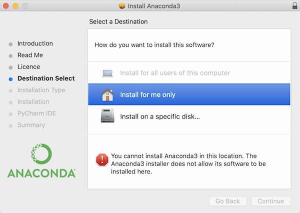
Once you’ve downloaded the installer, execute it and follow the on screen instructions. On MacOS, you might see the error message shown below. If you do, just re-select Install for me only and it should clear the error.
Starting Jupyter
Open up a command shell in your operating system. Create a new directory
(e.g. dsc_test) and cd to that directory to get started. Now start Jupyter
Notebook:-
jupyter notebookJupyter Notebook runs a web server and the User Interface is served as a web page. The Jupyter Notebook web page should open automatically in a browser window, when run locally. If not, note the URL, which will be printed at the command prompt and paste it in a browser window. By default, Jupyter Notebook runs on localhost:8888. You must leave the server running while you are working with Notebook. Do not close the command prompt window. Open another command prompt if you need to interact with a shell.
You will see the Jupyter user interface and a message that tells you
The Notebook List is empty. Click on the New button on the right side of
the window and select Python 3 to create a new notebook. Your new notebook
will open and you will find yourself in the Jupyter Notebook editor. The name
of the new notebook defaults to Untitled, which can be seen in the top line
of the window. Click on it to rename your notebook (e.g. First Notebook).
Your notebook will be saved in a file with extension .ipynb in the directory
where you started the server (e.g. "~/dsc_test/First Notebook.ipynb").
Notebook Layout
Notebooks are multi-modal, multi-media documents. They are composed of cells, where each cell contains content of a particular type. Some cells contain text, such as documentation and commentary. Other cells contain executable programs or program snippets. Quite often, the output of the program is contained within the cell, for example a table or graph of results. Python is the language most commonly used for programs, although other languages and scripts are supported.
The menu and toolbar allow us to do the most common tasks, such as creating or deleting a cell, executing the code in a cell, copying and pasting, etc. There are keyboard shortcuts for most commands and you can see these by clicking the keyboard icon in the toolbar.
Cells are edited by clicking on them and typing. The currently selected cell
is outlined. A green outline indicates we are in edit mode and a blue outline
indicates not. A drop-down in the toolbar indicates what type of content the
cell contains. It defaults to code for new cells. In this post, we will
only use the code and markdown types.
Documenting the Notebook
When working with notebooks, it is typical to mix code with the documentation that describes what is being done at each point. Markdown is the most common format used for this. If you are not familiar with Markdown, Github provides a useful introduction on their site github markdown reference.
Let’s add a title to our notebook. Select the first cell on the page and set
it’s type to markdown, using the drop-down list in the toolbar. Now, click
inside the cell to select edit mode and type in some h1 text.
# Jupyter Notebook Example 1Note that the editor interprets the markdown and gives you some sense of how it
will look in a completed notebook. Clicking on Run or hitting Shift-Enter
will show the actual formatted markdown. Double clicking on the cell will
return to edit mode.
Let’s add another cell below the first one and add some descriptive text about the purpose of this particular notebook.
Adding Code
Now we’re going to add some Python code. It is beyond the scope of this post to cover coding in Python and we would refer you to the web site if you’d like to learn Python.
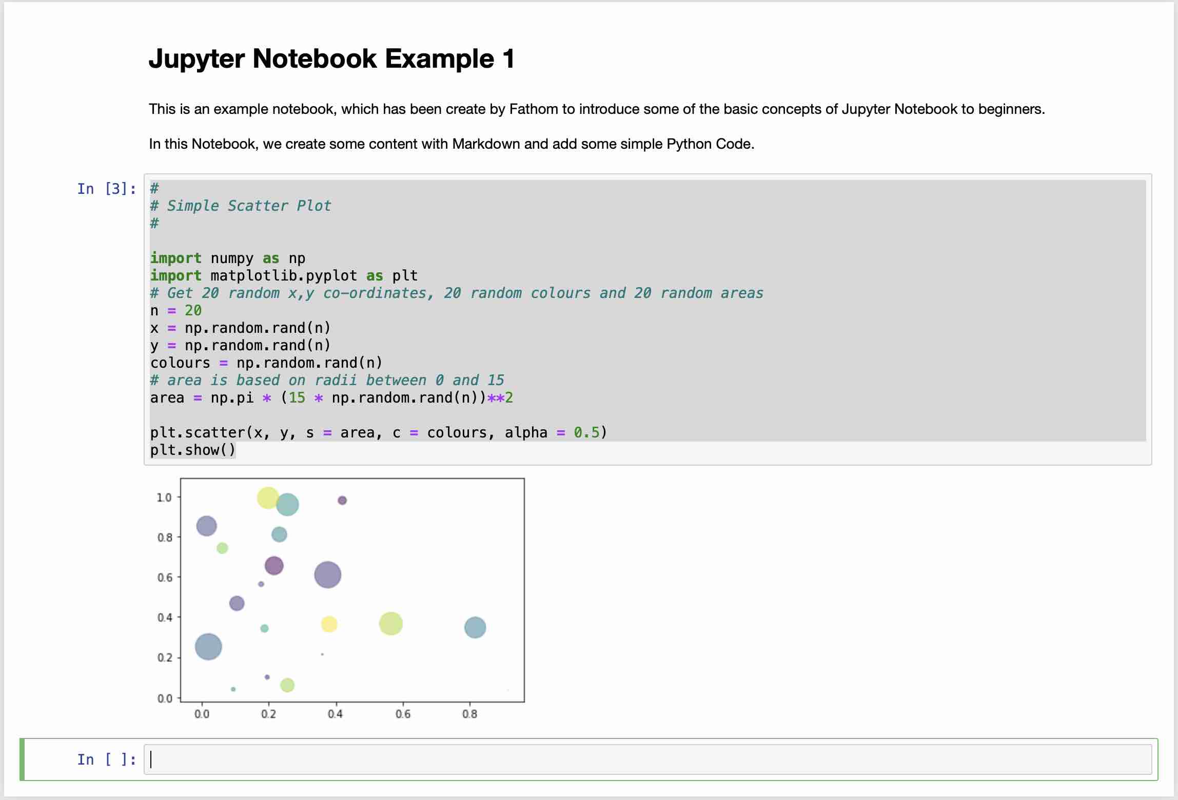
The sample code produces some output in the form of a plot of some data. For
the purposes of demonstration, we are going to generate some random data and
plot it. Paste the code below into a new cell of type code.
#
# Simple Scatter Plot
#

import numpy as np
import matplotlib.pyplot as plt
# Get 20 random x,y co-ordinates, 20 random colours and 20 random areas
n = 20
x = np.random.rand(n)
y = np.random.rand(n)
colours = np.random.rand(n)
# area is based on radii between 0 and 15
area = np.pi * (15 * np.random.rand(n))**2

plt.scatter(x, y, s = area, c = colours, alpha = 0.5)
plt.show()
The code uses two libraries that are commonly used in data science, numpy and
matplotlib. These libraries will have already been installed if you’ve been
following the installation using Anaconda. If you’ve installed Python by some
other method, you may need to install these with pip. Once you’ve pasted in
the code, go ahead and run it. You should see a scatter graph of random data.
At this point, your new Jupyter Notebook should look something like this:-
Finishing Up
So that’s it, you’ve created your first notebook with Jupyter Notebook.
Notebook updates are automatically saved in the .ipynb file but you can make
sure by click on the save icon in the toolbar. To exit, click on Close and Halt
in the File menu. Once you’ve closed the Notebook, you can go ahead and close
the browser window and return to the command prompt running the server and exit
that by hitting Ctrl-C. You can return to you notebook at any time by running
the server from the same directory where your notebook is saved and re-running
jupyter notebook and then selecting the notebook from the list of notebooks.
What’s Next
Hopefully, this brief introduction has whetted your appetite and you’ll want to explore further. We encourage you to explore Python at their site and some of the available data science libraries such as numpy and matplotlib.
We also encourage you to explore some of the other things you can do in notebooks. For example, you can add HTML to cells, allowing you to embed images or Video. You can insert other programming or scripting languages, such as Javascript or Shell Scripts. You can use MathJax in markdown cells to add mathematical or chemical equations to your documentation.
Because notebooks are stored in a simple JSON file format, they can easily be
shared, with many open source notebooks freely shared on the web. We encourage
you to explore resources such as
Jupyter Gallery.
Most of the examples are in Github. To download them you can clone the relevant
Github repository or simply grab an individual file. Because Github
automatically renders notebooks, you’ll need to view the file in Raw mode
and copy its contents into a text editor. Once your file is downloaded
and saved with a .ipyn extension, simply copy it into the folder where you
run Jupyter. It will now show up in your list of notebooks and you’ll be able
to open it for editing and running.
Hopefully, you’ll develop some interesting notebooks of your own that you can share with the community.